14 minutes
Building Distribution Reference Tables in R
I’ve recently been studing for a professional exam that does not allow computers or advanced calculators. Some of the subject matter will require use of a few statistical distributions which can be very time-consuming to calculate manually. In lieu of access to statistical functions, you are allowed to bring books and some reference sheets. I wanted to see if I could recreate these distribution tables in R.
Generating distribution values is very simple in R. The d, q, p, and r
functions are all that you will need to fill in the table values. The table
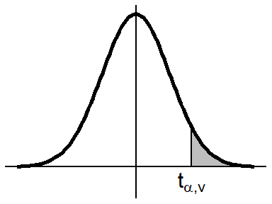
below is for the t distribution.
alpha <- c(.1, .05, .025, .01, .005)
v <- c(seq(1, 30, by = 1), Inf)
tTable <- sapply((1-alpha), function(x) qt(x, df = v))
colnames(tTable) <- alpha
I’m using the
xtable package here to format my table. It has some handy options to
parse math symbols and notations with its sanitize.text print options and allows
more customization of table style than the kable function in knitr. I’m
setting some of style options below.
options(xtable.type = 'html',
        xtable.caption.placement = "top",
        xtable.include.rownames = FALSE,
        xtable.html.table.attributes= list("border='2' cellpadding='15' cellpadding='5' rules ='all' width ='100%'"))
When rendering the table, you can use LaTeX notation within the data of the table and have it parsed into math notation.
library(xtable)

tTable <- data.frame("$v \\big\\backslash \\alpha$" = paste0("", v, ""),
                     tTable,
                     stringsAsFactors = FALSE,
                     check.names = FALSE)
tTable[[1]][tTable[[1]] == "Inf"] <- "$\\infty$"
tTable <- xtable(tTable,
                      caption = "Table 3: Percentiles of the *t* Distribution",
                      align = rep("c", ncol(tTable)+1),
                      digits = 4)
print(tTable)
| `\(v \big\backslash \alpha\)` | 0.1 | 0.05 | 0.025 | 0.01 | 0.005 |
|---|---|---|---|---|---|
| 1 | 3.0777 | 6.3138 | 12.7062 | 31.8205 | 63.6567 |
| 2 | 1.8856 | 2.9200 | 4.3027 | 6.9646 | 9.9248 |
| 3 | 1.6377 | 2.3534 | 3.1824 | 4.5407 | 5.8409 |
| 4 | 1.5332 | 2.1318 | 2.7764 | 3.7469 | 4.6041 |
| 5 | 1.4759 | 2.0150 | 2.5706 | 3.3649 | 4.0321 |
| 6 | 1.4398 | 1.9432 | 2.4469 | 3.1427 | 3.7074 |
| 7 | 1.4149 | 1.8946 | 2.3646 | 2.9980 | 3.4995 |
| 8 | 1.3968 | 1.8595 | 2.3060 | 2.8965 | 3.3554 |
| 9 | 1.3830 | 1.8331 | 2.2622 | 2.8214 | 3.2498 |
| 10 | 1.3722 | 1.8125 | 2.2281 | 2.7638 | 3.1693 |
| 11 | 1.3634 | 1.7959 | 2.2010 | 2.7181 | 3.1058 |
| 12 | 1.3562 | 1.7823 | 2.1788 | 2.6810 | 3.0545 |
| 13 | 1.3502 | 1.7709 | 2.1604 | 2.6503 | 3.0123 |
| 14 | 1.3450 | 1.7613 | 2.1448 | 2.6245 | 2.9768 |
| 15 | 1.3406 | 1.7531 | 2.1314 | 2.6025 | 2.9467 |
| 16 | 1.3368 | 1.7459 | 2.1199 | 2.5835 | 2.9208 |
| 17 | 1.3334 | 1.7396 | 2.1098 | 2.5669 | 2.8982 |
| 18 | 1.3304 | 1.7341 | 2.1009 | 2.5524 | 2.8784 |
| 19 | 1.3277 | 1.7291 | 2.0930 | 2.5395 | 2.8609 |
| 20 | 1.3253 | 1.7247 | 2.0860 | 2.5280 | 2.8453 |
| 21 | 1.3232 | 1.7207 | 2.0796 | 2.5176 | 2.8314 |
| 22 | 1.3212 | 1.7171 | 2.0739 | 2.5083 | 2.8188 |
| 23 | 1.3195 | 1.7139 | 2.0687 | 2.4999 | 2.8073 |
| 24 | 1.3178 | 1.7109 | 2.0639 | 2.4922 | 2.7969 |
| 25 | 1.3163 | 1.7081 | 2.0595 | 2.4851 | 2.7874 |
| 26 | 1.3150 | 1.7056 | 2.0555 | 2.4786 | 2.7787 |
| 27 | 1.3137 | 1.7033 | 2.0518 | 2.4727 | 2.7707 |
| 28 | 1.3125 | 1.7011 | 2.0484 | 2.4671 | 2.7633 |
| 29 | 1.3114 | 1.6991 | 2.0452 | 2.4620 | 2.7564 |
| 30 | 1.3104 | 1.6973 | 2.0423 | 2.4573 | 2.7500 |
| `\(\infty\)` | 1.2816 | 1.6449 | 1.9600 | 2.3263 | 2.5758 |
I also wanted to include a plot of the distribution and describe what the values
are visually. ?mathplot provides a guide to writing math notation in
expression to show math notation in plots. More information on how the math
notation will look is available
here.
library(ggplot2)

x <- seq(-3.5, 3.5, by = .001)
ggplot() +
  geom_ribbon(aes(x = seq(qnorm(.95), max(x), by = .001),
                  ymin = 0,
                  ymax = dnorm(seq(qnorm(.95), max(x), by = .001))),
              fill = 'gray') +
  geom_vline(xintercept = 0, color = "black") +
  geom_hline(yintercept = 0, color = "black") +
  stat_function(data = data.frame(x=x),aes(x = x),
                fun = dnorm,
                size = 1) +
  geom_segment(aes(x = qnorm(.95),
                   y = 0,
                   xend = qnorm(.95),
                   yend = dnorm(qnorm(.95))
  ),

  color = 'black') +
  theme_void() +
  theme(plot.margin = unit(c(.1,.1,.1,.1), "cm")) +
  annotate(geom = 'text',
           x = c(qnorm(.95)),
           y = c(-.04),
           label = c(expression(t[paste(alpha,',',v)])),
           size = 4,
           parse = TRUE) +
  coord_cartesian(ylim = c(-.06, dnorm(qnorm(.5))))
Below, is the code for the rest of the tables. I’ve also placed a printable version here.
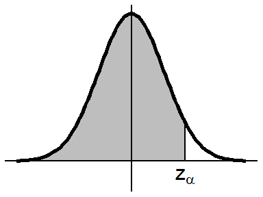
\(\text{Normal Distribution}\)
x <- seq(-3.5, 3.5, by = .001)
ggplot() +
  geom_ribbon(aes(x = seq(min(x), qnorm(.95), by = .001),
                  ymin = 0,
                  ymax = dnorm(seq(min(x), qnorm(.95), by = .001))),
              fill = 'gray') +
  geom_vline(xintercept = 0, color = "black") +
  geom_hline(yintercept = 0, color = "black") +
  stat_function(data = data.frame(x=x),aes(x = x),
                fun = dnorm,
                size = 1) +
  geom_segment(aes(x = qnorm(.95),
                   y = 0,
                   xend = qnorm(.95),
                   yend = dnorm(qnorm(.95))
  ),

  color = 'black') +
  theme_void() +
  theme(plot.margin = unit(c(.1,.1,.1,.1), "cm")) +
  annotate(geom = 'text',
           x = c(qnorm(.95)),
           y = c(-.04),
           label = c(expression(z[alpha])),
           size = 4,
           parse = TRUE) +
  coord_cartesian(ylim = c(-.06, dnorm(qnorm(.5))))
normalTable <- matrix(round(pnorm(seq(0, 3.49, by = .01)), 4),
                      ncol = 10,
                      byrow = TRUE)
colnames(normalTable) <- seq(0, .09, by = .01)
z <- sprintf("%01.1f", seq(0, 3.4, by = .1))
normalTable <- data.frame("$z$" = paste0("", z, ""),
                          normalTable,
                          stringsAsFactors = FALSE)
colnames(normalTable) <- c("z", seq(0, .09, by = .01))
normalTable <- xtable(normalTable,
                      caption = "Table 2: Cumulative Probabilities of the Standard Normal Distribution, $X \\sim N(0,1)$",
                      align = rep("c", ncol(normalTable)+1),
                      digits = 4)
print(normalTable)
| z | 0 | 0.01 | 0.02 | 0.03 | 0.04 | 0.05 | 0.06 | 0.07 | 0.08 | 0.09 |
|---|---|---|---|---|---|---|---|---|---|---|
| 0.0 | 0.5000 | 0.5040 | 0.5080 | 0.5120 | 0.5160 | 0.5199 | 0.5239 | 0.5279 | 0.5319 | 0.5359 |
| 0.1 | 0.5398 | 0.5438 | 0.5478 | 0.5517 | 0.5557 | 0.5596 | 0.5636 | 0.5675 | 0.5714 | 0.5753 |
| 0.2 | 0.5793 | 0.5832 | 0.5871 | 0.5910 | 0.5948 | 0.5987 | 0.6026 | 0.6064 | 0.6103 | 0.6141 |
| 0.3 | 0.6179 | 0.6217 | 0.6255 | 0.6293 | 0.6331 | 0.6368 | 0.6406 | 0.6443 | 0.6480 | 0.6517 |
| 0.4 | 0.6554 | 0.6591 | 0.6628 | 0.6664 | 0.6700 | 0.6736 | 0.6772 | 0.6808 | 0.6844 | 0.6879 |
| 0.5 | 0.6915 | 0.6950 | 0.6985 | 0.7019 | 0.7054 | 0.7088 | 0.7123 | 0.7157 | 0.7190 | 0.7224 |
| 0.6 | 0.7257 | 0.7291 | 0.7324 | 0.7357 | 0.7389 | 0.7422 | 0.7454 | 0.7486 | 0.7517 | 0.7549 |
| 0.7 | 0.7580 | 0.7611 | 0.7642 | 0.7673 | 0.7704 | 0.7734 | 0.7764 | 0.7794 | 0.7823 | 0.7852 |
| 0.8 | 0.7881 | 0.7910 | 0.7939 | 0.7967 | 0.7995 | 0.8023 | 0.8051 | 0.8078 | 0.8106 | 0.8133 |
| 0.9 | 0.8159 | 0.8186 | 0.8212 | 0.8238 | 0.8264 | 0.8289 | 0.8315 | 0.8340 | 0.8365 | 0.8389 |
| 1.0 | 0.8413 | 0.8438 | 0.8461 | 0.8485 | 0.8508 | 0.8531 | 0.8554 | 0.8577 | 0.8599 | 0.8621 |
| 1.1 | 0.8643 | 0.8665 | 0.8686 | 0.8708 | 0.8729 | 0.8749 | 0.8770 | 0.8790 | 0.8810 | 0.8830 |
| 1.2 | 0.8849 | 0.8869 | 0.8888 | 0.8907 | 0.8925 | 0.8944 | 0.8962 | 0.8980 | 0.8997 | 0.9015 |
| 1.3 | 0.9032 | 0.9049 | 0.9066 | 0.9082 | 0.9099 | 0.9115 | 0.9131 | 0.9147 | 0.9162 | 0.9177 |
| 1.4 | 0.9192 | 0.9207 | 0.9222 | 0.9236 | 0.9251 | 0.9265 | 0.9279 | 0.9292 | 0.9306 | 0.9319 |
| 1.5 | 0.9332 | 0.9345 | 0.9357 | 0.9370 | 0.9382 | 0.9394 | 0.9406 | 0.9418 | 0.9429 | 0.9441 |
| 1.6 | 0.9452 | 0.9463 | 0.9474 | 0.9484 | 0.9495 | 0.9505 | 0.9515 | 0.9525 | 0.9535 | 0.9545 |
| 1.7 | 0.9554 | 0.9564 | 0.9573 | 0.9582 | 0.9591 | 0.9599 | 0.9608 | 0.9616 | 0.9625 | 0.9633 |
| 1.8 | 0.9641 | 0.9649 | 0.9656 | 0.9664 | 0.9671 | 0.9678 | 0.9686 | 0.9693 | 0.9699 | 0.9706 |
| 1.9 | 0.9713 | 0.9719 | 0.9726 | 0.9732 | 0.9738 | 0.9744 | 0.9750 | 0.9756 | 0.9761 | 0.9767 |
| 2.0 | 0.9772 | 0.9778 | 0.9783 | 0.9788 | 0.9793 | 0.9798 | 0.9803 | 0.9808 | 0.9812 | 0.9817 |
| 2.1 | 0.9821 | 0.9826 | 0.9830 | 0.9834 | 0.9838 | 0.9842 | 0.9846 | 0.9850 | 0.9854 | 0.9857 |
| 2.2 | 0.9861 | 0.9864 | 0.9868 | 0.9871 | 0.9875 | 0.9878 | 0.9881 | 0.9884 | 0.9887 | 0.9890 |
| 2.3 | 0.9893 | 0.9896 | 0.9898 | 0.9901 | 0.9904 | 0.9906 | 0.9909 | 0.9911 | 0.9913 | 0.9916 |
| 2.4 | 0.9918 | 0.9920 | 0.9922 | 0.9925 | 0.9927 | 0.9929 | 0.9931 | 0.9932 | 0.9934 | 0.9936 |
| 2.5 | 0.9938 | 0.9940 | 0.9941 | 0.9943 | 0.9945 | 0.9946 | 0.9948 | 0.9949 | 0.9951 | 0.9952 |
| 2.6 | 0.9953 | 0.9955 | 0.9956 | 0.9957 | 0.9959 | 0.9960 | 0.9961 | 0.9962 | 0.9963 | 0.9964 |
| 2.7 | 0.9965 | 0.9966 | 0.9967 | 0.9968 | 0.9969 | 0.9970 | 0.9971 | 0.9972 | 0.9973 | 0.9974 |
| 2.8 | 0.9974 | 0.9975 | 0.9976 | 0.9977 | 0.9977 | 0.9978 | 0.9979 | 0.9979 | 0.9980 | 0.9981 |
| 2.9 | 0.9981 | 0.9982 | 0.9982 | 0.9983 | 0.9984 | 0.9984 | 0.9985 | 0.9985 | 0.9986 | 0.9986 |
| 3.0 | 0.9987 | 0.9987 | 0.9987 | 0.9988 | 0.9988 | 0.9989 | 0.9989 | 0.9989 | 0.9990 | 0.9990 |
| 3.1 | 0.9990 | 0.9991 | 0.9991 | 0.9991 | 0.9992 | 0.9992 | 0.9992 | 0.9992 | 0.9993 | 0.9993 |
| 3.2 | 0.9993 | 0.9993 | 0.9994 | 0.9994 | 0.9994 | 0.9994 | 0.9994 | 0.9995 | 0.9995 | 0.9995 |
| 3.3 | 0.9995 | 0.9995 | 0.9995 | 0.9996 | 0.9996 | 0.9996 | 0.9996 | 0.9996 | 0.9996 | 0.9997 |
| 3.4 | 0.9997 | 0.9997 | 0.9997 | 0.9997 | 0.9997 | 0.9997 | 0.9997 | 0.9997 | 0.9997 | 0.9998 |
\(t \text{ Distribution}\)
x <- seq(-3.5, 3.5, by = .001)
ggplot() +
  geom_ribbon(aes(x = seq(qnorm(.95), max(x), by = .001),
                  ymin = 0,
                  ymax = dnorm(seq(qnorm(.95), max(x), by = .001))),
              fill = 'gray') +
  geom_vline(xintercept = 0, color = "black") +
  geom_hline(yintercept = 0, color = "black") +
  stat_function(data = data.frame(x=x),aes(x = x),
                fun = dnorm,
                size = 1) +
  geom_segment(aes(x = qnorm(.95),
                   y = 0,
                   xend = qnorm(.95),
                   yend = dnorm(qnorm(.95))
  ),

  color = 'black') +
  theme_void() +
  theme(plot.margin = unit(c(.1,.1,.1,.1), "cm")) +
  annotate(geom = 'text',
           x = c(qnorm(.95)),
           y = c(-.04),
           label = c(expression(t[paste(alpha,',',v)])),
           size = 4,
           parse = TRUE) +
  coord_cartesian(ylim = c(-.06, dnorm(qnorm(.5))))

alpha <- c(.1, .05, .025, .01, .005)
v <- c(seq(1, 30, by = 1), Inf)
tTable <- sapply((1-alpha), function(x) qt(x, df = v))
colnames(tTable) <- alpha
tTable <- data.frame("$v \\big\\backslash \\alpha$" = paste0("", v, ""),
                     tTable,
                     stringsAsFactors = FALSE,
                     check.names = FALSE)
tTable[[1]][tTable[[1]] == "Inf"] <- "$\\infty$"
tTable <- xtable(tTable,
                      caption = "Table 3: Percentiles of the *t* Distribution",
                      align = rep("c", ncol(tTable)+1),
                      digits = 4)
print(tTable)
| `\(v \big\backslash \alpha\)` | 0.1 | 0.05 | 0.025 | 0.01 | 0.005 |
|---|---|---|---|---|---|
| 1 | 3.0777 | 6.3138 | 12.7062 | 31.8205 | 63.6567 |
| 2 | 1.8856 | 2.9200 | 4.3027 | 6.9646 | 9.9248 |
| 3 | 1.6377 | 2.3534 | 3.1824 | 4.5407 | 5.8409 |
| 4 | 1.5332 | 2.1318 | 2.7764 | 3.7469 | 4.6041 |
| 5 | 1.4759 | 2.0150 | 2.5706 | 3.3649 | 4.0321 |
| 6 | 1.4398 | 1.9432 | 2.4469 | 3.1427 | 3.7074 |
| 7 | 1.4149 | 1.8946 | 2.3646 | 2.9980 | 3.4995 |
| 8 | 1.3968 | 1.8595 | 2.3060 | 2.8965 | 3.3554 |
| 9 | 1.3830 | 1.8331 | 2.2622 | 2.8214 | 3.2498 |
| 10 | 1.3722 | 1.8125 | 2.2281 | 2.7638 | 3.1693 |
| 11 | 1.3634 | 1.7959 | 2.2010 | 2.7181 | 3.1058 |
| 12 | 1.3562 | 1.7823 | 2.1788 | 2.6810 | 3.0545 |
| 13 | 1.3502 | 1.7709 | 2.1604 | 2.6503 | 3.0123 |
| 14 | 1.3450 | 1.7613 | 2.1448 | 2.6245 | 2.9768 |
| 15 | 1.3406 | 1.7531 | 2.1314 | 2.6025 | 2.9467 |
| 16 | 1.3368 | 1.7459 | 2.1199 | 2.5835 | 2.9208 |
| 17 | 1.3334 | 1.7396 | 2.1098 | 2.5669 | 2.8982 |
| 18 | 1.3304 | 1.7341 | 2.1009 | 2.5524 | 2.8784 |
| 19 | 1.3277 | 1.7291 | 2.0930 | 2.5395 | 2.8609 |
| 20 | 1.3253 | 1.7247 | 2.0860 | 2.5280 | 2.8453 |
| 21 | 1.3232 | 1.7207 | 2.0796 | 2.5176 | 2.8314 |
| 22 | 1.3212 | 1.7171 | 2.0739 | 2.5083 | 2.8188 |
| 23 | 1.3195 | 1.7139 | 2.0687 | 2.4999 | 2.8073 |
| 24 | 1.3178 | 1.7109 | 2.0639 | 2.4922 | 2.7969 |
| 25 | 1.3163 | 1.7081 | 2.0595 | 2.4851 | 2.7874 |
| 26 | 1.3150 | 1.7056 | 2.0555 | 2.4786 | 2.7787 |
| 27 | 1.3137 | 1.7033 | 2.0518 | 2.4727 | 2.7707 |
| 28 | 1.3125 | 1.7011 | 2.0484 | 2.4671 | 2.7633 |
| 29 | 1.3114 | 1.6991 | 2.0452 | 2.4620 | 2.7564 |
| 30 | 1.3104 | 1.6973 | 2.0423 | 2.4573 | 2.7500 |
| `\(\infty\)` | 1.2816 | 1.6449 | 1.9600 | 2.3263 | 2.5758 |
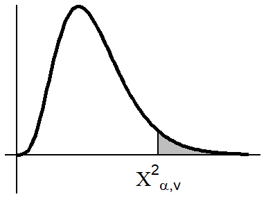
\(\chi^2 \text{ Distribution}\)
x <- seq(0, 30, .01)
v <- 10
ggplot() +
  geom_ribbon(aes(x = seq(qchisq(.95, df = v), max(x), by = .001),
                  ymin = 0,
                  ymax = dchisq(seq(qchisq(.95, df = v), max(x), by = .001),
                                df = v)
                  ),
              fill = 'gray') +
  geom_vline(xintercept = 0, color = "black") +
  geom_hline(yintercept = 0, color = "black") +
  stat_function(data = data.frame(x=x),aes(x = x),
                fun = dchisq,
                args = list(df = v),
                size = 1) +
  geom_segment(aes(x = qchisq(.95, df = v),
                   y = 0,
                   xend = qchisq(.95, df = v),
                   yend = dchisq(qchisq(.95, df = v), df = v)
  ),

  color = 'black') +
  theme_void() +
  theme(plot.margin = unit(c(.1,.1,.1,.1), "cm")) +
  annotate(geom = 'text',
           x = c(qchisq(.95, df = v)),
           y = c(-.015),
           label = c(expression( paste(Chi^2)[paste(alpha,',','v')])),
           size = 4,
           parse = TRUE) +
  coord_cartesian(ylim = c(-.02, dchisq(qchisq(.5, df = v), df = v)))
| `\(v \big\backslash \alpha\)` | 0.995 | 0.99 | 0.975 | 0.95 | 0.9 | 0.75 | 0.5 | 0.25 | 0.1 | 0.05 | 0.025 | 0.01 | 0.005 | 0.001 |
|---|---|---|---|---|---|---|---|---|---|---|---|---|---|---|
| 1 | 0.00 | 0.00 | 0.00 | 0.00 | 0.02 | 0.10 | 0.45 | 1.32 | 2.71 | 3.84 | 5.02 | 6.63 | 7.88 | 10.83 |
| 2 | 0.01 | 0.02 | 0.05 | 0.10 | 0.21 | 0.58 | 1.39 | 2.77 | 4.61 | 5.99 | 7.38 | 9.21 | 10.60 | 13.82 |
| 3 | 0.07 | 0.11 | 0.22 | 0.35 | 0.58 | 1.21 | 2.37 | 4.11 | 6.25 | 7.81 | 9.35 | 11.34 | 12.84 | 16.27 |
| 4 | 0.21 | 0.30 | 0.48 | 0.71 | 1.06 | 1.92 | 3.36 | 5.39 | 7.78 | 9.49 | 11.14 | 13.28 | 14.86 | 18.47 |
| 5 | 0.41 | 0.55 | 0.83 | 1.15 | 1.61 | 2.67 | 4.35 | 6.63 | 9.24 | 11.07 | 12.83 | 15.09 | 16.75 | 20.52 |
| 6 | 0.68 | 0.87 | 1.24 | 1.64 | 2.20 | 3.45 | 5.35 | 7.84 | 10.64 | 12.59 | 14.45 | 16.81 | 18.55 | 22.46 |
| 7 | 0.99 | 1.24 | 1.69 | 2.17 | 2.83 | 4.25 | 6.35 | 9.04 | 12.02 | 14.07 | 16.01 | 18.48 | 20.28 | 24.32 |
| 8 | 1.34 | 1.65 | 2.18 | 2.73 | 3.49 | 5.07 | 7.34 | 10.22 | 13.36 | 15.51 | 17.53 | 20.09 | 21.95 | 26.12 |
| 9 | 1.73 | 2.09 | 2.70 | 3.33 | 4.17 | 5.90 | 8.34 | 11.39 | 14.68 | 16.92 | 19.02 | 21.67 | 23.59 | 27.88 |
| 10 | 2.16 | 2.56 | 3.25 | 3.94 | 4.87 | 6.74 | 9.34 | 12.55 | 15.99 | 18.31 | 20.48 | 23.21 | 25.19 | 29.59 |
| 11 | 2.60 | 3.05 | 3.82 | 4.57 | 5.58 | 7.58 | 10.34 | 13.70 | 17.28 | 19.68 | 21.92 | 24.72 | 26.76 | 31.26 |
| 12 | 3.07 | 3.57 | 4.40 | 5.23 | 6.30 | 8.44 | 11.34 | 14.85 | 18.55 | 21.03 | 23.34 | 26.22 | 28.30 | 32.91 |
| 13 | 3.57 | 4.11 | 5.01 | 5.89 | 7.04 | 9.30 | 12.34 | 15.98 | 19.81 | 22.36 | 24.74 | 27.69 | 29.82 | 34.53 |
| 14 | 4.07 | 4.66 | 5.63 | 6.57 | 7.79 | 10.17 | 13.34 | 17.12 | 21.06 | 23.68 | 26.12 | 29.14 | 31.32 | 36.12 |
| 15 | 4.60 | 5.23 | 6.26 | 7.26 | 8.55 | 11.04 | 14.34 | 18.25 | 22.31 | 25.00 | 27.49 | 30.58 | 32.80 | 37.70 |
| 16 | 5.14 | 5.81 | 6.91 | 7.96 | 9.31 | 11.91 | 15.34 | 19.37 | 23.54 | 26.30 | 28.85 | 32.00 | 34.27 | 39.25 |
| 17 | 5.70 | 6.41 | 7.56 | 8.67 | 10.09 | 12.79 | 16.34 | 20.49 | 24.77 | 27.59 | 30.19 | 33.41 | 35.72 | 40.79 |
| 18 | 6.26 | 7.01 | 8.23 | 9.39 | 10.86 | 13.68 | 17.34 | 21.60 | 25.99 | 28.87 | 31.53 | 34.81 | 37.16 | 42.31 |
| 19 | 6.84 | 7.63 | 8.91 | 10.12 | 11.65 | 14.56 | 18.34 | 22.72 | 27.20 | 30.14 | 32.85 | 36.19 | 38.58 | 43.82 |
| 20 | 7.43 | 8.26 | 9.59 | 10.85 | 12.44 | 15.45 | 19.34 | 23.83 | 28.41 | 31.41 | 34.17 | 37.57 | 40.00 | 45.31 |
| 21 | 8.03 | 8.90 | 10.28 | 11.59 | 13.24 | 16.34 | 20.34 | 24.93 | 29.62 | 32.67 | 35.48 | 38.93 | 41.40 | 46.80 |
| 22 | 8.64 | 9.54 | 10.98 | 12.34 | 14.04 | 17.24 | 21.34 | 26.04 | 30.81 | 33.92 | 36.78 | 40.29 | 42.80 | 48.27 |
| 23 | 9.26 | 10.20 | 11.69 | 13.09 | 14.85 | 18.14 | 22.34 | 27.14 | 32.01 | 35.17 | 38.08 | 41.64 | 44.18 | 49.73 |
| 24 | 9.89 | 10.86 | 12.40 | 13.85 | 15.66 | 19.04 | 23.34 | 28.24 | 33.20 | 36.42 | 39.36 | 42.98 | 45.56 | 51.18 |
| 25 | 10.52 | 11.52 | 13.12 | 14.61 | 16.47 | 19.94 | 24.34 | 29.34 | 34.38 | 37.65 | 40.65 | 44.31 | 46.93 | 52.62 |
| 30 | 13.79 | 14.95 | 16.79 | 18.49 | 20.60 | 24.48 | 29.34 | 34.80 | 40.26 | 43.77 | 46.98 | 50.89 | 53.67 | 59.70 |
| 40 | 20.71 | 22.16 | 24.43 | 26.51 | 29.05 | 33.66 | 39.34 | 45.62 | 51.81 | 55.76 | 59.34 | 63.69 | 66.77 | 73.40 |
| 50 | 27.99 | 29.71 | 32.36 | 34.76 | 37.69 | 42.94 | 49.33 | 56.33 | 63.17 | 67.50 | 71.42 | 76.15 | 79.49 | 86.66 |
| 60 | 35.53 | 37.48 | 40.48 | 43.19 | 46.46 | 52.29 | 59.33 | 66.98 | 74.40 | 79.08 | 83.30 | 88.38 | 91.95 | 99.61 |
| 70 | 43.28 | 45.44 | 48.76 | 51.74 | 55.33 | 61.70 | 69.33 | 77.58 | 85.53 | 90.53 | 95.02 | 100.43 | 104.21 | 112.32 |
| 80 | 51.17 | 53.54 | 57.15 | 60.39 | 64.28 | 71.14 | 79.33 | 88.13 | 96.58 | 101.88 | 106.63 | 112.33 | 116.32 | 124.84 |
| 90 | 59.20 | 61.75 | 65.65 | 69.13 | 73.29 | 80.62 | 89.33 | 98.65 | 107.57 | 113.15 | 118.14 | 124.12 | 128.30 | 137.21 |
| 100 | 67.33 | 70.06 | 74.22 | 77.93 | 82.36 | 90.13 | 99.33 | 109.14 | 118.50 | 124.34 | 129.56 | 135.81 | 140.17 | 149.45 |
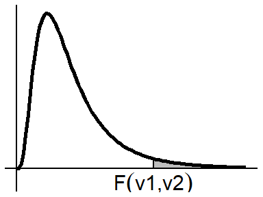
\(F(v_1, v_2) \text{ Distribution}\)
x <- seq(0, 5, .01)
v1 <- 10
v2 <- 10
ggplot() +
  geom_ribbon(aes(x = seq(qf(.95, df1 = v1, df2 = v2), max(x), by = .001),
                  ymin = 0,
                  ymax = df(seq(qf(.95, df1 = v1, df2 = v2), max(x), by = .001),
                                df1 = v1, df2 = v2)
                  ),
              fill = 'gray') +
  geom_vline(xintercept = 0, color = "black") +
  geom_hline(yintercept = 0, color = "black") +
  stat_function(data = data.frame(x=x),aes(x = x),
                fun = df,
                args = list(df1 = v1, df2 = v2),
                size = 1) +
  geom_segment(aes(x = qf(.95, df1 = v1, df2 = v2),
                   y = 0,
                   xend = qf(.95, df1 = v1, df2 = v2),
                   yend = df(qf(.95, df1 = v1, df2 = v2), df1 = v1, df2 = v2)
  ),

  color = 'black') +
  theme_void() +
  theme(plot.margin = unit(c(.1,.1,.1,.1), "cm")) +
  annotate(geom = 'text',
           x = c(qf(.95, df1 = v1, df2 = v2)),
           y = c(-.07),
           label = c(expression(F(paste(v1,',',v2)))),
           size = 4,
           parse = TRUE) +
  coord_cartesian(ylim = c(-.07, df(qf(.25, df1 = v1, df2 = v2), df1 = v1, df2 = v2)))
v1 <- c(seq(1, 10, by = 1), 12, 15, 20, 24, 30, 40, 60, 120, Inf)
v2 <- v1
fTable95 <- sapply(v1, function(x) round(qf(.95, x, v2), 2))
colnames(fTable95) <- v1
colnames(fTable95)[colnames(fTable95) == 'Inf'] <- "$\\infty$"
fTable95 <- data.frame("$v_2 \\big\\backslash v_1$" = paste0("", v2, ""),
                       fTable95,
                       stringsAsFactors = FALSE,
                       check.names = FALSE)
fTable95[[1]][fTable95[[1]] == "Inf"] <- "$\\infty$"
fTable95 <- xtable(fTable95,
                      caption = "Table 5: 95th Percentiles of the $F(v_1,v_2)$",
                      align = rep("c", ncol(fTable95)+1))

print(fTable95)
| `\(v_2 \big\backslash v_1\)` | 1 | 2 | 3 | 4 | 5 | 6 | 7 | 8 | 9 | 10 | 12 | 15 | 20 | 24 | 30 | 40 | 60 | 120 | `\(\infty\)` |
|---|---|---|---|---|---|---|---|---|---|---|---|---|---|---|---|---|---|---|---|
| 1 | 161.45 | 199.50 | 215.71 | 224.58 | 230.16 | 233.99 | 236.77 | 238.88 | 240.54 | 241.88 | 243.91 | 245.95 | 248.01 | 249.05 | 250.10 | 251.14 | 252.20 | 253.25 | 254.31 |
| 2 | 18.51 | 19.00 | 19.16 | 19.25 | 19.30 | 19.33 | 19.35 | 19.37 | 19.38 | 19.40 | 19.41 | 19.43 | 19.45 | 19.45 | 19.46 | 19.47 | 19.48 | 19.49 | 19.50 |
| 3 | 10.13 | 9.55 | 9.28 | 9.12 | 9.01 | 8.94 | 8.89 | 8.85 | 8.81 | 8.79 | 8.74 | 8.70 | 8.66 | 8.64 | 8.62 | 8.59 | 8.57 | 8.55 | 8.53 |
| 4 | 7.71 | 6.94 | 6.59 | 6.39 | 6.26 | 6.16 | 6.09 | 6.04 | 6.00 | 5.96 | 5.91 | 5.86 | 5.80 | 5.77 | 5.75 | 5.72 | 5.69 | 5.66 | 5.63 |
| 5 | 6.61 | 5.79 | 5.41 | 5.19 | 5.05 | 4.95 | 4.88 | 4.82 | 4.77 | 4.74 | 4.68 | 4.62 | 4.56 | 4.53 | 4.50 | 4.46 | 4.43 | 4.40 | 4.36 |
| 6 | 5.99 | 5.14 | 4.76 | 4.53 | 4.39 | 4.28 | 4.21 | 4.15 | 4.10 | 4.06 | 4.00 | 3.94 | 3.87 | 3.84 | 3.81 | 3.77 | 3.74 | 3.70 | 3.67 |
| 7 | 5.59 | 4.74 | 4.35 | 4.12 | 3.97 | 3.87 | 3.79 | 3.73 | 3.68 | 3.64 | 3.57 | 3.51 | 3.44 | 3.41 | 3.38 | 3.34 | 3.30 | 3.27 | 3.23 |
| 8 | 5.32 | 4.46 | 4.07 | 3.84 | 3.69 | 3.58 | 3.50 | 3.44 | 3.39 | 3.35 | 3.28 | 3.22 | 3.15 | 3.12 | 3.08 | 3.04 | 3.01 | 2.97 | 2.93 |
| 9 | 5.12 | 4.26 | 3.86 | 3.63 | 3.48 | 3.37 | 3.29 | 3.23 | 3.18 | 3.14 | 3.07 | 3.01 | 2.94 | 2.90 | 2.86 | 2.83 | 2.79 | 2.75 | 2.71 |
| 10 | 4.96 | 4.10 | 3.71 | 3.48 | 3.33 | 3.22 | 3.14 | 3.07 | 3.02 | 2.98 | 2.91 | 2.85 | 2.77 | 2.74 | 2.70 | 2.66 | 2.62 | 2.58 | 2.54 |
| 12 | 4.75 | 3.89 | 3.49 | 3.26 | 3.11 | 3.00 | 2.91 | 2.85 | 2.80 | 2.75 | 2.69 | 2.62 | 2.54 | 2.51 | 2.47 | 2.43 | 2.38 | 2.34 | 2.30 |
| 15 | 4.54 | 3.68 | 3.29 | 3.06 | 2.90 | 2.79 | 2.71 | 2.64 | 2.59 | 2.54 | 2.48 | 2.40 | 2.33 | 2.29 | 2.25 | 2.20 | 2.16 | 2.11 | 2.07 |
| 20 | 4.35 | 3.49 | 3.10 | 2.87 | 2.71 | 2.60 | 2.51 | 2.45 | 2.39 | 2.35 | 2.28 | 2.20 | 2.12 | 2.08 | 2.04 | 1.99 | 1.95 | 1.90 | 1.84 |
| 24 | 4.26 | 3.40 | 3.01 | 2.78 | 2.62 | 2.51 | 2.42 | 2.36 | 2.30 | 2.25 | 2.18 | 2.11 | 2.03 | 1.98 | 1.94 | 1.89 | 1.84 | 1.79 | 1.73 |
| 30 | 4.17 | 3.32 | 2.92 | 2.69 | 2.53 | 2.42 | 2.33 | 2.27 | 2.21 | 2.16 | 2.09 | 2.01 | 1.93 | 1.89 | 1.84 | 1.79 | 1.74 | 1.68 | 1.62 |
| 40 | 4.08 | 3.23 | 2.84 | 2.61 | 2.45 | 2.34 | 2.25 | 2.18 | 2.12 | 2.08 | 2.00 | 1.92 | 1.84 | 1.79 | 1.74 | 1.69 | 1.64 | 1.58 | 1.51 |
| 60 | 4.00 | 3.15 | 2.76 | 2.53 | 2.37 | 2.25 | 2.17 | 2.10 | 2.04 | 1.99 | 1.92 | 1.84 | 1.75 | 1.70 | 1.65 | 1.59 | 1.53 | 1.47 | 1.39 |
| 120 | 3.92 | 3.07 | 2.68 | 2.45 | 2.29 | 2.18 | 2.09 | 2.02 | 1.96 | 1.91 | 1.83 | 1.75 | 1.66 | 1.61 | 1.55 | 1.50 | 1.43 | 1.35 | 1.25 |
| `\(\infty\)` | 3.84 | 3.00 | 2.60 | 2.37 | 2.21 | 2.10 | 2.01 | 1.94 | 1.88 | 1.83 | 1.75 | 1.67 | 1.57 | 1.52 | 1.46 | 1.39 | 1.32 | 1.22 | 1.00 |