You contribute to the reference sheet here: https://github.com/tomroh/pe_ise_prep.

Systems Definition, Analysis, and Design

System Analysis and Design Tools

Cause-Effect Diagram (Fishbone)

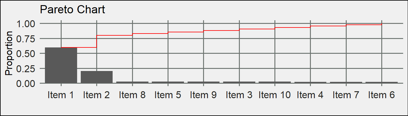
Pareto Analysis

80% of the items represent 20% of the sales or 20% of the items represent 80% of the cost. This law is a rule of thumb.

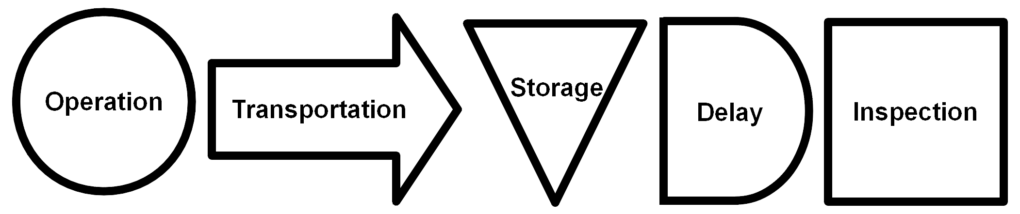
Operation Process Chart

The operation process chart only has Operations and Inspections.

Flow Process Chart

The flow process chart forces a more detailed look at a system.

Affinity Diagram

organizes a large number of ideas into their natural relationships

Left Hand Right Hand Chart

Shows when each hand is busy and idle. It is sometimes called a simo chart.

Modeling Techniques

Queueing Models

$$Littl{e}^{\prime }sLaw$$

---

$$L=\lambda W$$

$M/M/c/KQueue$

---

Effective vs. Offered Load:

$${\lambda }_{eff}=\lambda (1-{\pi }_m)$$

Waiting Time Law:

$$L=\sum _{n=0}^{M}n{\pi }_n$$ $$L_q=\sum _{n=c+1}^{c-1}(n-c){\pi }_n$$

Probability of n arrivals by time t:

$$P[N(t)=n]=\frac{(\lambda t{)}^n{e}^{-\lambda t}}{n!}$$

$M/M/1/\mathrm{\infty }Queue$

---

Probability of customers in system:

$${\pi }_0=1-\rho$$ $${\pi }_n={\rho }^n(1-\rho )$$ $$L=\frac{\rho }{1-\rho }$$ $$L_q=L-\rho =\frac{{\rho }^2}{1-\rho }$$

$M/G/1/\mathrm{\infty }Queue$

---

Pollaczek-Khintchine Formula:

$$L=L_q+\rho =\frac{{\rho }^2+{\lambda }^2{\sigma }^2}{2(1-\rho )}+\rho$$

$M/M/c/MQueue$

---

$$D=\sum _{n=0}^{c-1}\frac{{\rho }^n}{n!}+\frac{{\rho }^c}{c!}[\frac{1-(\rho /c{)}^{M-c+1}}{1-\rho /c}]$$ $${\pi }_0=\frac{1}{D}$$

$${\pi }_n=\{\begin{array}{l}\frac{{\rho }^n}{n!}{\pi }_0,\text{n<c}\\ \frac{{\rho }^n}{c!c^{n-c}}{\pi }_0,n\ge c\end{array}$$

$$L_q={\pi }_0(\frac{{\rho }^{c+1}}{(c-1)!(c-\rho {)}^2})[1-(\frac{\rho }{c}{)}^{M-c}-(M-c)(\frac{\rho }{c}{)}^{M-c}(1-\frac{\rho }{c})],\rho \ne c$$

$$L_q={\pi }_0(\frac{{\rho }^c(M-c)(M-c+1)}{2c!}),\rho =c$$

$$L_q={\pi }_0(\frac{{\rho }^{c+1}}{(c-1)!(c-\rho {)}^2}),c=\mathrm{\infty }$$

$M/M/C/\mathrm{\infty }Queue$

---

C = 1

$$P_0=1-\rho ,L_q=\frac{{\rho }^2}{1-\rho }$$

C = 2

$$P_0=\frac{(1-\rho )}{(1=\rho },L_q=\frac{2{\rho }^3}{(1-{\rho }^2)}$$

C = 3

$$P_0=\frac{2(1-\rho )}{2+4\rho +3{\rho }^2},\frac{9{\rho }^4}{2+2\rho -{\rho }^2-3{\rho }^3}$$

Model Verification

A model has been verified if a range of models produce similar results on the same situation

Model Validation

A model has been validated if a range of results produce similar results on the same situation

Bottleneck Analysis

Optimize the process that is the bottleneck, then re-evaulate the bottleneck and repeat.

Facilities Engineering and Planning

People/Equipment Requirements

$$M_j=\sum _{i=1}^n\frac{P_{ij}{T}_{ij}}{C_{ij}}$$ $$\begin{gathered} M_j=\text{number of machines/people} \\ P=\text{production rate} \\ T=\text{production time} \\ C=\text{production period} \\ n=\text{number of products} \end{gathered}$$

Material Handling

Euclidian:

$$d=\sqrt{(x_2-x_1{)}^2+(y_2-y_1{)}^2}$$

To optimize material flow:

$$min\sum _{i=1}^m{w}_i[(x-a_i{)}^2+(y-b_i){]}^{\frac{1}{2}}$$ If there are 4 locations with equal weight, the optimal location is the facility within a triangle of the other facilities. If there is no such facility, the optimal location is at the intersection of two lines.

When the weighted costs are proportional to the square of the Euclidean distance, it is called the ‘gravity’ problem.

$$min\sum _{i=1}^m{w}_i[(x-a_i{)}^2+(y-b_i{)}^2]$$

$$x=\frac{\sum _{i=1}^m{w}_i{a}_i}{\sum _{i=1}^m{w}_i}$$ $$y=\frac{\sum _{i=1}^m{w}_i{b}_i}{\sum _{i=1}^m{w}_i}$$

Manhattan:

$$|x_2-x_1|+|y_2-y_1|$$

To optimize flow:

$$min\sum _{i=1}^m{w}_i(|x-a_1|+|y-b_i|)$$

The x value is the median of the location x-coordinates. The y value is the median of the location y-coordinates.

Chebyshev (simultaneous x and y movement)

$$max(|x_2-x_1|,|y_2-y_1|)$$

Relationship Chart

Code	Closeness	Rank
A	Absolutely Necessary	0.95
E	Especially Important	0.85
I	Important	0.7
O	Ordinary Closeness	0.5
U	Unimportant	0
X	Not desirable	-

Supply Chain Logistics

Forecasting Methods

Moving Average

$${\hat{d}}_t=\frac{\sum _{i=1}^n{d}_{t-i}}{n}$$

Exponentially Weighted Moving Average

$$\begin{gathered} {\hat{d}}_t=\alpha d_{t-1}+(1-\alpha ){\hat{d}}_{t-1},0\le \alpha (\text{smoothing constant})\le 1 \\ {d}_{t-1}\text{ = actual demand, }{\hat{d}}_{t-1}\text{ = forecasted demand} \end{gathered}$$

Production Planning Methods

Systems to compute Master Production and Ordering Plan

Material Requirements Planning (MRP)

Manufacturing Resource Planning (MRPII)

Engineering Economics

$$\begin{gathered} (\frac{F}{P})=(1+i{)}^N,(\frac{P}{F})=\frac{1}{(1+i{)}^N} \\ (\frac{F}{A})=\frac{(1+i{)}^N-1}{i},(\frac{P}{A})=\frac{(1+i{)}^N-1}{i(1+i{)}^N} \\ (\frac{A}{F})=\frac{i}{(1+i{)}^N-1},(\frac{A}{P})=\frac{i(1+i{)}^N}{(1+i{)}^N-1} \\ (\frac{P}{G})=\frac{1}{i}[\frac{(1+i{)}^N-1}{i(1+i{)}^N}-\frac{N}{(1+i{)}^N}],(\frac{A}{G})=\frac{1}{i}-\frac{N}{(1+i{)}^N-1} \end{gathered}$$

*Denominator is current value and Numerator is desired conversion

Depreciation

Modified Accelerated Cost Recovery System (MACRS) - See Tables

$$\text{Straight Line (SL) - }\frac{1}{n}$$

Production Scheduling Methods

Makespan

the time it takes from the start of the first job until the end of the last job

Scheduling Sequence

1. Earliest Due Date - order jobs by due date
2. Shortest Processing Time - order jobs by processing time
3. Critical Ratio - divide time remaining until due date by time left on the machine, order by smallest critical ratio

Johnson’s Optimal Rule for Two Machines

1. Find the shortest processsing times and arbitrarily break ties
2. If the shortest processing time is on Machine A, schedule immediately. If the shortest processing time is on Machine B, schedule it as late as possible.
3. Eliminate the last job scheduled on the list and repeat step 1-2.

Inventory Management and Control

Economic Order Quantity

$$\begin{gathered} Q^{\ast }=\sqrt{\frac{2C_{p}D}{h}R} \\ R=\frac{1}{1-\frac{D}{P}},\text{R=1, when replenishment is instaneous} \\ D=\text{demand},P=\text{production rate},C_p=\text{cost per order},h=\text{holding cost} \end{gathered}$$

Economic Manufacturing Quantity

Use the equation above with R not equal to 1.

With shortage costs

$$\begin{gathered} Q^{\ast }=\sqrt{\frac{2C_{p}D}{h}R(\frac{h+z}{z})} \\ z=\text{shortage cost} \end{gathered}$$

$$\begin{gathered} M^{\ast }=\sqrt{\frac{2C_{p}D(1-\frac{D}{P})h}{z(h+z)}} \\ M=\text{allowed shortage} \end{gathered}$$

Carrying Cost

$$C_T=\frac{hQ}{2}(1-\frac{D}{P})+CD+C_p\frac{D}{Q}$$

Probabilistic Inventory and Production Models

$$\begin{gathered} F_D(x=y^{\ast })\ge \frac{p-c}{p+h} \\ {F}_D=\text{CDF} \\ x=\text{units on hand},y^{\ast }=\text{optimal order quantity},p=\text{loss of potential revenue}, \\ h=\text{loss in value from holding},c=\text{unit acquisition cost} \end{gathered}$$

Distribution Methods

Transhipment:

The intermediary storage

Transportation Problem

$$\begin{gathered} min\sum _{i=1}^m\sum _{j=1}^n{x}_{ij}{c}_{ij} \\ \sum _{j=1}^n{x}_{ij}=s_i,n=1,2,...,m \\ \sum _{i=1}^m{x}_{ij}=d_j,m=1,2,...,n \end{gathered}$$

Storage and Warehousing Methods

1. Dedicated Storage
   • easy to retrieve items
   • Sum of maximum of each product
2. Random Storage
   • more efficient use of space
   • Maximum of the sums of all products

Transportation Modes

1. Variable Path
   • truck, vehicle anything that does not have one fixed path
   • versatility
2. Fixed Path
   • conveyor
   • tied to one path

Assignment Problem

Hungarian Procedure:

1. Subtract the minimum of the row from all elements in the row
2. Substract the minimum of the column from all elements in the columns
3. Try to make a valid assignment using the zero elements, if all assigments cannot be made proceed to next step
4. Cover all zeroes with the minimal number of lines
5. From each uncovered element subtract the minimum of the uncovered y, add y to each intersection element. Go to step 3.
6. Transfer the assignment plan to the original cost table.

Work Design

Controls

An administrative control are training, policies, or procedures.

An engineering control is a physical modification to mitigate hazards.

Noise Dose

Dose

$$D=100\ast (\frac{C_1}{T_1}+\frac{C_2}{T_2}+...+\frac{C_n}{T_n})\le 100$$

Time Weighted Average

$$TWA=16.61lo{g}_{10}(\frac{D}{100})+90$$

Exposure

Time Weighted Concentration

$$TWA=\frac{\sum _{i=1}^n{C}_i{T}_i}{\sum _{i=1}^n{T}_i}$$

Taylor Tool Life

$$\begin{gathered} V{T}^n=C \\ V=\text{speed surface feet per minute} \\ T=\text{tool life in minutes} \\ C,n=\text{constants that depend on material and tool} \end{gathered}$$

Work Sampling

$$\begin{gathered} D=Z_{\alpha /2}\sqrt{\frac{p(-1-p)}{n}},Z_{\alpha /2}\sqrt{\frac{1-p}{pn}} \\ p=\text{proportion of observed time} \\ D=\text{absolute error} \\ R=\text{relative error}=\frac{D}{p} \\ n=\text{sample size} \end{gathered}$$

Sample Size

$$E=\frac{z_{\frac{\alpha }{2}}\sigma }{\sqrt{n}}$$

$$n=(\frac{z_{\frac{\alpha }{2}}\sigma }{E}{)}^2$$

Critical Path Method

$$T=\sum _{(i,j)\in CP}{d}_{ij}$$

Standard Time

$$\text{Observed Time * Pace Rating * (1 + personal time allowance) * (1 + fatigue allowance)}$$

Recommended Weight Limit

Units are pounds and inches.

$$\begin{gathered} RWL=51\cdot (\frac{10}{H})\cdot (1-.0075|V-30|)\cdot (.82+\frac{1.8}{D})\cdot (1-.0032A)\cdot FM\cdot CM \\ \text{H = horizontal location of the load forward of the midpoint of the ankles} \\ \text{V = vertical location of the load} \\ \text{D = Vertical travel distance between the origin and the destination} \\ \text{A=angle of asymmetry between hands and feet} \\ \text{FM = frequency multiplier (from table)} \\ \text{CM = coupling mulitiplier (from table)} \end{gathered}$$

Learning Curve

$$\begin{gathered} y=k{x}^n,n=\frac{lo{g}_e\varphi }{lo{g}_e(2)} \\ \varphi =\text{learning ratio}=\frac{T(2N)}{T(N)},\text{T(N) = time to produce Nth unit} \\ \text{y= time to produce xth unit, k = time to produce first unit, x = cumulative number of units produced} \end{gathered}$$

Total Learning Time:

$$T=k\frac{[(x_2+\frac{1}{2}{)}^{n+1}-(x_1+\frac{1}{2}{)}^{n+1}]}{n+1}$$

Remission Line:

$$y=k+\frac{(k-s)(x-1)}{1-x_s}$$

Quality Control

Statistical Process Control

X & R-Chart

$$\begin{gathered} UCL=D_4\overline{R} \\ CL=\overline{R} \\ LCL=D_3\overline{R} \end{gathered}$$

$$\begin{gathered} UCL=\overline{\overline{X}}+A_2\overline{R} \\ CL=\overline{\overline{X}} \\ LCL=\overline{\overline{X}}-A_2\overline{R} \end{gathered}$$

X & S-Chart

$$\begin{gathered} UCL=B_4\overline{S} \\ CL=\overline{X} \\ LCL=B_3\overline{S} \end{gathered}$$

$$\begin{gathered} UCL=\overline{\overline{X}}+A_3\overline{S} \\ CL=\overline{\overline{X}} \\ LCL=\overline{\overline{X}}-A_3\overline{S} \end{gathered}$$

P-Chart

$$\begin{gathered} UCL=\overline{p}+3\sqrt{\frac{\overline{p}(1-\overline{p})}{n}} \\ CL=\overline{p} \\ LCL=\overline{p}-3\sqrt{\frac{\overline{p}(1-\overline{p})}{n}} \end{gathered}$$

C-Chart

$$\begin{gathered} UCL=\overline{c}+3\sqrt{\overline{c}} \\ CL=\overline{c} \\ LCL=\overline{c}-3\sqrt{\overline{c}} \end{gathered}$$

Tests for Out of Control

1. A single point falls outside three sigma control limits
2. Two out of three successive points fall on the same side of and more than two sigma units from the center line
3. Four out of five successive points fall on the same side of and more than one sigma unit from the center line
4. Eight successive points fall on the same side of the center line

Control vs. Capability

In control if it is within natural variability

Is capable if it is entirely within specification

Process Capability

Actual Capability:

$$C_{pk}=min(\frac{\mu -LSL}{3\sigma },\frac{USL-\mu }{3\sigma })$$

Potential Capability:

$$C_p=\frac{USL-LSL}{6\sigma }$$

Reliability Analysis

Series:

$$R=\prod _{i=1}^n{P}_i$$

Parallel:

$$R=1-\prod _{i=1}^n(1-P_i)$$

Hazard Function

$$\begin{gathered} h(x)=\frac{f(x)}{R(x)} \\ f(x)\text{ = density function, }R(x)\text{ = survival function} \end{gathered}$$

Exponential $$h(x)=\lambda$$

Weibull $$h(x)=\frac{\beta }{\alpha }(\frac{x}{\alpha }{)}^{\beta -1}$$

Mean Time to Failure

$$\begin{gathered} \frac{1}{\lambda }, \\ \lambda \text{ = constant failure rate} \end{gathered}$$

Six Sigma

`$\sigma$`	Defects per Million
1.00	158655.254
1.50	66807.201
2.00	22750.132
2.50	6209.665
3.00	1349.898
3.50	232.629
4.00	31.671
4.50	3.398
5.00	0.287
5.50	0.019
6.00	0.001

Statistics

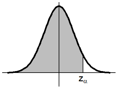
Normal Distribution

z-score

$$z=\frac{x-\mu }{\sigma }$$

Confidence Interval

$$\overline{x}\pm \frac{z_{\alpha /2}\sigma }{\sqrt{n}}$$

Two-means comparison:

$$z_0=\frac{{\overline{x}}_1-{\overline{x}}_2}{\sqrt{\frac{{\sigma }_1^2}{n_1}+\frac{{\sigma }_2^2}{n_2}}}$$

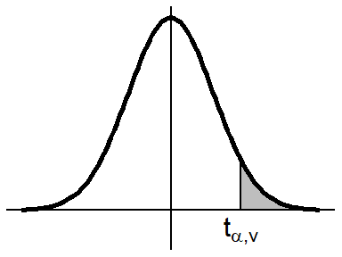
student-t Distribution

t-score:

$$t=\frac{\overline{x}-\mu }{\frac{s}{\sqrt{n}}}$$

Confidence Interval

$$\overline{x}\pm \frac{t_{\alpha /2,n-1}s}{\sqrt{n}}$$

Two-means comparison:

$$t_0=\frac{{\overline{x}}_1-{\overline{x}}_2}{\sqrt{\frac{s_1^2}{n_1}+\frac{s_2^2}{n_2}}}$$

df for Two Sample t-test:

$$df=\frac{(\frac{s_1^2}{n_1}+\frac{s_2^2}{n_2}{)}^2}{\frac{(\frac{s_1^2}{n_1}{)}^2}{n_1-1}+\frac{(\frac{s_1^2}{n_1}{)}^2}{n_1-1}}$$ Paired t-test:

$$t_0=\frac{\overline{d}-0}{\frac{s_d}{\sqrt{n}}}$$

Hypothesis Testing

Error Table

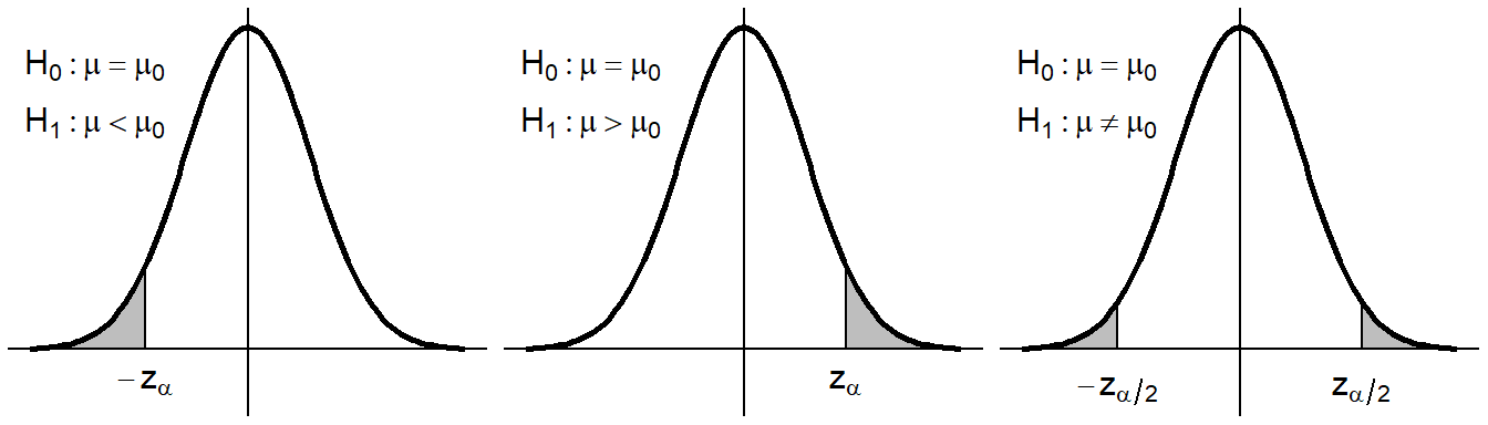
	`$H_0\text{ is true}$`	`$H_0\text{ is false}$`
`$\text{Accept }{H}_0$`	Correct	Type II Error
`$\text{Reject }{H}_0$`	Type I Error	Correct

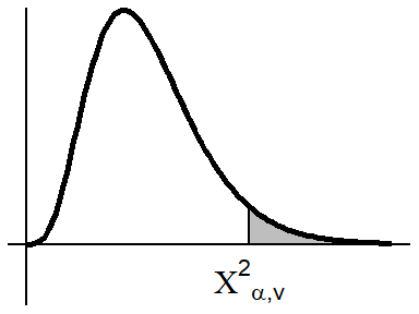
Chi-Squared Goodness of Fit

$${\chi }^2=\sum _{j=1}^k\frac{(O_j-E_j{)}^2}{E_j}$$

Linear Regression

$$SSR=\sum _{i=1}^n({\hat{y}}_i-\overline{y}{)}^2$$

$$SSE=\sum _{i=1}^n(y_i-{\hat{y}}_i{)}^2$$

$$SST=\sum _{i=1}^n(y_i-\overline{y}{)}^2$$

$$R^2=\frac{SSR}{SST}=1-\frac{SSE}{SST}$$

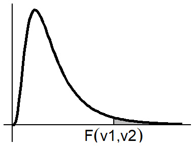
ANOVA

$$SSA+SSE=SST$$

One-Way

Given Treatment A:

$$SSA+SSE=SST$$

SS	df	MS	F
SSA	a-1	SSA/dfA	MSA/MSE
SSE	a(n-1)	SSE/dfE
SST	an-1

Two-Way

Given treatment factors A & B:

$$SST=SSA+SSB+SSAB+SSE$$

SS	df	MS	F
SSA	a-1	SSA/dfA	MSA/MSE
SSB	b-1	SSB/dfB	MSB/MSE
SSAB	(a-1)(b-1)	SSAB/dfAB	MSAB/MSE
SSE	ab(n-1)	SSE/dfE
SST	abn-1

Bayesian Analysis

Bayes' Theorem

$$P(A|B)=\frac{P(B|A)P(A)}{P(B)}=\frac{P(B|A)P(A)}{P(B|A)P(A)+P(B|A^{\prime })P(A^{\prime })}$$

Distributions

Discrete

Distribution	pmf	cdf	mean	variance	parameters
Binomial	`$(\genfrac{}{}{0ex}{}{n}{x})p^x(1-p{)}^{n-x}$`	`$\sum _{i=0}^{\lfloor x\rfloor }(\genfrac{}{}{0ex}{}{n}{i})p^i(1-p{)}^{n-i}$`	`$np$`	`$np(1-p)$`	`$$\begin{gathered} \text{n = number of trials} \\ \text{p = success probability} \end{gathered}$$`
Discrete Uniform	`$\frac{1}{b-a+1}$`	`$\frac{\lfloor x\rfloor -a+1}{b-a+1}$`	`$\frac{a+b}{2}$`	`$\frac{(b-a+1{)}^2-1}{12}$`	`$$\begin{gathered} \text{a = minimum} \\ \text{b = maximum} \end{gathered}$$`
Poisson	`$\frac{{\lambda }^x{e}^{-\lambda }}{x!}$`	`$e^{-\lambda }\sum _{i=0}^{\lfloor x\rfloor }\frac{{\lambda }^i}{i!}$`	`$\lambda$`	`$\lambda$`	`$\lambda \text{ = rate}$`
Geometric	`$p(1-p{)}^x$`	`$1-(1-p{)}^{x+1}$`	`$\frac{1-p}{p}$`	`$\frac{1-p}{p^2}$`	`$$\begin{gathered} \text{k = number of trials} \\ \text{p = success probability} \end{gathered}$$`
Negative Binomial	`$(\genfrac{}{}{0ex}{}{k+x-1}{x})p^k(1-p{)}^x$`	`$-$`	`$\frac{k(1-p)}{p}$`	`$\frac{k(1-p)}{p^2}$`	`$$\begin{gathered} \text{k = number of successes} \\ \text{p = success probability} \end{gathered}$$`

Continuous

Distribution	pdf	cdf	mean	variance	parameters
Uniform	`$\frac{1}{b-a}$`	`$\frac{x-a}{b-a}$`	`$\frac{a+b}{2}$`	`$\frac{(b-a{)}^2}{12}$`	`$$\begin{gathered} \text{a = minimum} \\ \text{b = maximum} \end{gathered}$$`
Exponential	`$\lambda e^{-\lambda x}$`	`$1-e^{-\lambda x}$`	`$\frac{1}{\lambda }$`	`$\frac{1}{{\lambda }^2}$`	`$\lambda \text{ = rate}$`
Normal	`$\frac{1}{\sqrt{2\pi {\sigma }^2}}{e}^{-\frac{(x-\mu {)}^2}{2{\sigma }^2}}$`	`$\frac{1}{2}[1+erf(\frac{x-\mu }{\sigma \sqrt{2}})]$`	`$\mu$`	`${\sigma }^2$`	`$$\begin{gathered} \mu \text{ = mean} \\ {\sigma }^2\text{ = variance} \end{gathered}$$`
PERT beta	`$-$`	`$-$`	`$\frac{a+4m+b}{6}$`	`$\frac{(b-a{)}^2}{36}$`	`$$\begin{gathered} \text{a = 1st percentile} \\ \text{b = 99th percentile} \\ \text{m = mode} \end{gathered}$$`
Triangular	$\begin{cases} \frac{(x-a)^2}{(b-a)(c-a)},\quad a\le x\le c \ 1-\frac{(b-x)^2}{(b-a)(b-c)},\quad c	$\begin{cases} \frac{(x-a)^2}{(b-a)(c-a)},\quad a\le x\le c \ 1-\frac{(b-x)^2}{(b-a)(b-c)}, \quad c	`$\frac{a+b+c}{3}$`	`$\frac{a^2+m^2+b^2-ca-ab-cb}{18}$`	`$$\begin{gathered} \text{a = minimum} \\ \text{b = maximum} \\ \text{c = mode} \end{gathered}$$`
Gamma	`$\frac{{\beta }^{\alpha }}{\mathrm{\Gamma }(\alpha )}{x}^{\alpha -1}{e}^{-\beta x}$`	`$\frac{1}{\mathrm{\Gamma }(\alpha )}\gamma (\alpha ,\beta x)$`	`$\alpha \beta$`	`$\alpha {\beta }^2$`	`$$\begin{gathered} \alpha \text{ = shape} \\ \beta \text{ = scale} \end{gathered}$$`
Weibull	`$\frac{\beta }{\alpha }{(\genfrac{}{}{0ex}{}{x}{\alpha })}^{\beta -1}{e}^{-(\frac{x}{\alpha }{)}^{\beta }}$`	`$1-e^{-(\frac{x}{\alpha }{)}^{\beta }}$`	`$-$`	`$-$`	`$-$`
Lognormal	`$\frac{1}{x\sigma \sqrt{2\pi }}{e}^{\frac{(lnx-\mu {)}^2}{2{\sigma }^2}}$`	`$\frac{1}{2}+\frac{1}{2}erf[\frac{lnx-\mu }{\sigma \sqrt{2}}]$`	`$e^{\mu +\frac{{\sigma }^2}{2}}$`	`$[e^{{\sigma }^2}-1]e^{2\mu +{\sigma }^2}$`	`$$\begin{gathered} \mu \text{ = mean} \\ {\sigma }^2\text{ = variance} \end{gathered}$$`

$\text{Factors for Control Charts}$

Table 1: Factors for Calculating Limits for Variable Control Charts

`$n$`	`$A$`	`$A_2$`	`$A_3$`	`$c_4$`	`$B_3$`	`$B_4$`	`$B_5$`	`$B_6$`	`$d_2$`	`$d_2^{-1}$`	`$d_3$`	`$D_1$`	`$D_2$`	`$D_3$`	`$D_4$`
2	2.121	1.880	2.659	0.798	0.000	3.267	0.000	2.606	1.128	0.886	0.853	0.000	3.686	0.000	3.267
3	1.732	1.023	1.954	0.886	0.000	2.568	0.000	2.276	1.693	0.591	0.888	0.000	4.358	0.000	2.575
4	1.500	0.729	1.628	0.921	0.000	2.266	0.000	2.088	2.059	0.486	0.880	0.000	4.698	0.000	2.282
5	1.342	0.577	1.427	0.940	0.000	2.089	0.000	1.964	2.326	0.430	0.864	0.000	4.918	0.000	2.114
6	1.225	0.483	1.287	0.952	0.030	1.970	0.029	1.874	2.534	0.395	0.848	0.000	5.079	0.000	2.004
7	1.134	0.419	1.182	0.959	0.118	1.882	0.113	1.806	2.704	0.370	0.833	0.205	5.204	0.076	1.924
8	1.061	0.373	1.099	0.965	0.185	1.815	0.179	1.751	2.847	0.351	0.820	0.388	5.307	0.136	1.864
9	1.000	0.337	1.032	0.969	0.239	1.761	0.232	1.707	2.970	0.337	0.808	0.547	5.394	0.184	1.816
10	0.949	0.308	0.975	0.973	0.284	1.716	0.276	1.669	3.078	0.325	0.797	0.686	5.469	0.223	1.777
11	0.905	0.285	0.927	0.975	0.321	1.679	0.313	1.637	3.173	0.315	0.787	0.811	5.535	0.256	1.744
12	0.866	0.266	0.886	0.978	0.354	1.646	0.346	1.610	3.258	0.307	0.778	0.923	5.594	0.283	1.717
13	0.832	0.249	0.850	0.979	0.382	1.618	0.374	1.585	3.336	0.300	0.770	1.025	5.647	0.307	1.693
14	0.802	0.235	0.817	0.981	0.406	1.594	0.399	1.563	3.407	0.293	0.763	1.118	5.696	0.328	1.672
15	0.775	0.223	0.789	0.982	0.428	1.572	0.421	1.544	3.472	0.288	0.756	1.203	5.740	0.347	1.653
16	0.750	0.212	0.763	0.984	0.448	1.552	0.440	1.526	3.532	0.283	0.750	1.282	5.782	0.363	1.637
17	0.728	0.203	0.739	0.985	0.466	1.534	0.458	1.511	3.588	0.279	0.744	1.356	5.820	0.378	1.622
18	0.707	0.194	0.718	0.985	0.482	1.518	0.475	1.496	3.640	0.275	0.739	1.424	5.856	0.391	1.609
19	0.688	0.187	0.698	0.986	0.497	1.503	0.490	1.483	3.689	0.271	0.733	1.489	5.889	0.404	1.596
20	0.671	0.180	0.680	0.987	0.510	1.490	0.504	1.470	3.735	0.268	0.729	1.549	5.921	0.415	1.585
21	0.655	0.173	0.663	0.988	0.523	1.477	0.516	1.459	3.778	0.265	0.724	1.606	5.951	0.425	1.575
22	0.640	0.167	0.647	0.988	0.534	1.466	0.528	1.448	3.819	0.262	0.720	1.660	5.979	0.435	1.565
23	0.626	0.162	0.633	0.989	0.545	1.455	0.539	1.438	3.858	0.259	0.716	1.711	6.006	0.443	1.557
24	0.612	0.157	0.619	0.989	0.555	1.445	0.549	1.429	3.895	0.257	0.712	1.759	6.032	0.452	1.548
25	0.600	0.153	0.606	0.990	0.565	1.435	0.559	1.420	3.931	0.254	0.708	1.805	6.056	0.459	1.541

$\text{Normal Distribution}$

Table 2: Cumulative Probabilities of the Standard Normal Distribution, `$X\sim N(0,1)$`

z	0	0.01	0.02	0.03	0.04	0.05	0.06	0.07	0.08	0.09
0.0	0.5000	0.5040	0.5080	0.5120	0.5160	0.5199	0.5239	0.5279	0.5319	0.5359
0.1	0.5398	0.5438	0.5478	0.5517	0.5557	0.5596	0.5636	0.5675	0.5714	0.5753
0.2	0.5793	0.5832	0.5871	0.5910	0.5948	0.5987	0.6026	0.6064	0.6103	0.6141
0.3	0.6179	0.6217	0.6255	0.6293	0.6331	0.6368	0.6406	0.6443	0.6480	0.6517
0.4	0.6554	0.6591	0.6628	0.6664	0.6700	0.6736	0.6772	0.6808	0.6844	0.6879
0.5	0.6915	0.6950	0.6985	0.7019	0.7054	0.7088	0.7123	0.7157	0.7190	0.7224
0.6	0.7257	0.7291	0.7324	0.7357	0.7389	0.7422	0.7454	0.7486	0.7517	0.7549
0.7	0.7580	0.7611	0.7642	0.7673	0.7704	0.7734	0.7764	0.7794	0.7823	0.7852
0.8	0.7881	0.7910	0.7939	0.7967	0.7995	0.8023	0.8051	0.8078	0.8106	0.8133
0.9	0.8159	0.8186	0.8212	0.8238	0.8264	0.8289	0.8315	0.8340	0.8365	0.8389
1.0	0.8413	0.8438	0.8461	0.8485	0.8508	0.8531	0.8554	0.8577	0.8599	0.8621
1.1	0.8643	0.8665	0.8686	0.8708	0.8729	0.8749	0.8770	0.8790	0.8810	0.8830
1.2	0.8849	0.8869	0.8888	0.8907	0.8925	0.8944	0.8962	0.8980	0.8997	0.9015
1.3	0.9032	0.9049	0.9066	0.9082	0.9099	0.9115	0.9131	0.9147	0.9162	0.9177
1.4	0.9192	0.9207	0.9222	0.9236	0.9251	0.9265	0.9279	0.9292	0.9306	0.9319
1.5	0.9332	0.9345	0.9357	0.9370	0.9382	0.9394	0.9406	0.9418	0.9429	0.9441
1.6	0.9452	0.9463	0.9474	0.9484	0.9495	0.9505	0.9515	0.9525	0.9535	0.9545
1.7	0.9554	0.9564	0.9573	0.9582	0.9591	0.9599	0.9608	0.9616	0.9625	0.9633
1.8	0.9641	0.9649	0.9656	0.9664	0.9671	0.9678	0.9686	0.9693	0.9699	0.9706
1.9	0.9713	0.9719	0.9726	0.9732	0.9738	0.9744	0.9750	0.9756	0.9761	0.9767
2.0	0.9772	0.9778	0.9783	0.9788	0.9793	0.9798	0.9803	0.9808	0.9812	0.9817
2.1	0.9821	0.9826	0.9830	0.9834	0.9838	0.9842	0.9846	0.9850	0.9854	0.9857
2.2	0.9861	0.9864	0.9868	0.9871	0.9875	0.9878	0.9881	0.9884	0.9887	0.9890
2.3	0.9893	0.9896	0.9898	0.9901	0.9904	0.9906	0.9909	0.9911	0.9913	0.9916
2.4	0.9918	0.9920	0.9922	0.9925	0.9927	0.9929	0.9931	0.9932	0.9934	0.9936
2.5	0.9938	0.9940	0.9941	0.9943	0.9945	0.9946	0.9948	0.9949	0.9951	0.9952
2.6	0.9953	0.9955	0.9956	0.9957	0.9959	0.9960	0.9961	0.9962	0.9963	0.9964
2.7	0.9965	0.9966	0.9967	0.9968	0.9969	0.9970	0.9971	0.9972	0.9973	0.9974
2.8	0.9974	0.9975	0.9976	0.9977	0.9977	0.9978	0.9979	0.9979	0.9980	0.9981
2.9	0.9981	0.9982	0.9982	0.9983	0.9984	0.9984	0.9985	0.9985	0.9986	0.9986
3.0	0.9987	0.9987	0.9987	0.9988	0.9988	0.9989	0.9989	0.9989	0.9990	0.9990
3.1	0.9990	0.9991	0.9991	0.9991	0.9992	0.9992	0.9992	0.9992	0.9993	0.9993
3.2	0.9993	0.9993	0.9994	0.9994	0.9994	0.9994	0.9994	0.9995	0.9995	0.9995
3.3	0.9995	0.9995	0.9995	0.9996	0.9996	0.9996	0.9996	0.9996	0.9996	0.9997
3.4	0.9997	0.9997	0.9997	0.9997	0.9997	0.9997	0.9997	0.9997	0.9997	0.9998

$t\text{ Distribution}$

Table 3: Percentiles of the *t* Distribution

`$v\backslash \alpha$`	0.1	0.05	0.025	0.01	0.005
1	3.0777	6.3138	12.7062	31.8205	63.6567
2	1.8856	2.9200	4.3027	6.9646	9.9248
3	1.6377	2.3534	3.1824	4.5407	5.8409
4	1.5332	2.1318	2.7764	3.7469	4.6041
5	1.4759	2.0150	2.5706	3.3649	4.0321
6	1.4398	1.9432	2.4469	3.1427	3.7074
7	1.4149	1.8946	2.3646	2.9980	3.4995
8	1.3968	1.8595	2.3060	2.8965	3.3554
9	1.3830	1.8331	2.2622	2.8214	3.2498
10	1.3722	1.8125	2.2281	2.7638	3.1693
11	1.3634	1.7959	2.2010	2.7181	3.1058
12	1.3562	1.7823	2.1788	2.6810	3.0545
13	1.3502	1.7709	2.1604	2.6503	3.0123
14	1.3450	1.7613	2.1448	2.6245	2.9768
15	1.3406	1.7531	2.1314	2.6025	2.9467
16	1.3368	1.7459	2.1199	2.5835	2.9208
17	1.3334	1.7396	2.1098	2.5669	2.8982
18	1.3304	1.7341	2.1009	2.5524	2.8784
19	1.3277	1.7291	2.0930	2.5395	2.8609
20	1.3253	1.7247	2.0860	2.5280	2.8453
21	1.3232	1.7207	2.0796	2.5176	2.8314
22	1.3212	1.7171	2.0739	2.5083	2.8188
23	1.3195	1.7139	2.0687	2.4999	2.8073
24	1.3178	1.7109	2.0639	2.4922	2.7969
25	1.3163	1.7081	2.0595	2.4851	2.7874
26	1.3150	1.7056	2.0555	2.4786	2.7787
27	1.3137	1.7033	2.0518	2.4727	2.7707
28	1.3125	1.7011	2.0484	2.4671	2.7633
29	1.3114	1.6991	2.0452	2.4620	2.7564
30	1.3104	1.6973	2.0423	2.4573	2.7500
Inf	1.2816	1.6449	1.9600	2.3263	2.5758

${\chi }^2\text{ Distribution}$

Table 4: Percentiles of the `${\chi }^2$` Distribution

`$v\backslash \alpha$`	0.995	0.99	0.975	0.95	0.9	0.75	0.5	0.25	0.1	0.05	0.025	0.01	0.005	0.001
1	0.00	0.00	0.00	0.00	0.02	0.10	0.45	1.32	2.71	3.84	5.02	6.63	7.88	10.83
2	0.01	0.02	0.05	0.10	0.21	0.58	1.39	2.77	4.61	5.99	7.38	9.21	10.60	13.82
3	0.07	0.11	0.22	0.35	0.58	1.21	2.37	4.11	6.25	7.81	9.35	11.34	12.84	16.27
4	0.21	0.30	0.48	0.71	1.06	1.92	3.36	5.39	7.78	9.49	11.14	13.28	14.86	18.47
5	0.41	0.55	0.83	1.15	1.61	2.67	4.35	6.63	9.24	11.07	12.83	15.09	16.75	20.52
6	0.68	0.87	1.24	1.64	2.20	3.45	5.35	7.84	10.64	12.59	14.45	16.81	18.55	22.46
7	0.99	1.24	1.69	2.17	2.83	4.25	6.35	9.04	12.02	14.07	16.01	18.48	20.28	24.32
8	1.34	1.65	2.18	2.73	3.49	5.07	7.34	10.22	13.36	15.51	17.53	20.09	21.95	26.12
9	1.73	2.09	2.70	3.33	4.17	5.90	8.34	11.39	14.68	16.92	19.02	21.67	23.59	27.88
10	2.16	2.56	3.25	3.94	4.87	6.74	9.34	12.55	15.99	18.31	20.48	23.21	25.19	29.59
11	2.60	3.05	3.82	4.57	5.58	7.58	10.34	13.70	17.28	19.68	21.92	24.72	26.76	31.26
12	3.07	3.57	4.40	5.23	6.30	8.44	11.34	14.85	18.55	21.03	23.34	26.22	28.30	32.91
13	3.57	4.11	5.01	5.89	7.04	9.30	12.34	15.98	19.81	22.36	24.74	27.69	29.82	34.53
14	4.07	4.66	5.63	6.57	7.79	10.17	13.34	17.12	21.06	23.68	26.12	29.14	31.32	36.12
15	4.60	5.23	6.26	7.26	8.55	11.04	14.34	18.25	22.31	25.00	27.49	30.58	32.80	37.70
16	5.14	5.81	6.91	7.96	9.31	11.91	15.34	19.37	23.54	26.30	28.85	32.00	34.27	39.25
17	5.70	6.41	7.56	8.67	10.09	12.79	16.34	20.49	24.77	27.59	30.19	33.41	35.72	40.79
18	6.26	7.01	8.23	9.39	10.86	13.68	17.34	21.60	25.99	28.87	31.53	34.81	37.16	42.31
19	6.84	7.63	8.91	10.12	11.65	14.56	18.34	22.72	27.20	30.14	32.85	36.19	38.58	43.82
20	7.43	8.26	9.59	10.85	12.44	15.45	19.34	23.83	28.41	31.41	34.17	37.57	40.00	45.31
21	8.03	8.90	10.28	11.59	13.24	16.34	20.34	24.93	29.62	32.67	35.48	38.93	41.40	46.80
22	8.64	9.54	10.98	12.34	14.04	17.24	21.34	26.04	30.81	33.92	36.78	40.29	42.80	48.27
23	9.26	10.20	11.69	13.09	14.85	18.14	22.34	27.14	32.01	35.17	38.08	41.64	44.18	49.73
24	9.89	10.86	12.40	13.85	15.66	19.04	23.34	28.24	33.20	36.42	39.36	42.98	45.56	51.18
25	10.52	11.52	13.12	14.61	16.47	19.94	24.34	29.34	34.38	37.65	40.65	44.31	46.93	52.62
30	13.79	14.95	16.79	18.49	20.60	24.48	29.34	34.80	40.26	43.77	46.98	50.89	53.67	59.70
40	20.71	22.16	24.43	26.51	29.05	33.66	39.34	45.62	51.81	55.76	59.34	63.69	66.77	73.40
50	27.99	29.71	32.36	34.76	37.69	42.94	49.33	56.33	63.17	67.50	71.42	76.15	79.49	86.66
60	35.53	37.48	40.48	43.19	46.46	52.29	59.33	66.98	74.40	79.08	83.30	88.38	91.95	99.61
70	43.28	45.44	48.76	51.74	55.33	61.70	69.33	77.58	85.53	90.53	95.02	100.43	104.21	112.32
80	51.17	53.54	57.15	60.39	64.28	71.14	79.33	88.13	96.58	101.88	106.63	112.33	116.32	124.84
90	59.20	61.75	65.65	69.13	73.29	80.62	89.33	98.65	107.57	113.15	118.14	124.12	128.30	137.21
100	67.33	70.06	74.22	77.93	82.36	90.13	99.33	109.14	118.50	124.34	129.56	135.81	140.17	149.45

$F(v_1,v_2)\text{ Distribution}$

Table 5: 95th Percentiles of the `$F(v_1,v_2)$`

`$v_2\backslash v_1$`	1	2	3	4	5	6	7	8	9	10	12	15	20	24	30	40	60	120	`$\mathrm{\infty }$`
1	161.45	199.50	215.71	224.58	230.16	233.99	236.77	238.88	240.54	241.88	243.91	245.95	248.01	249.05	250.10	251.14	252.20	253.25	254.31
2	18.51	19.00	19.16	19.25	19.30	19.33	19.35	19.37	19.38	19.40	19.41	19.43	19.45	19.45	19.46	19.47	19.48	19.49	19.50
3	10.13	9.55	9.28	9.12	9.01	8.94	8.89	8.85	8.81	8.79	8.74	8.70	8.66	8.64	8.62	8.59	8.57	8.55	8.53
4	7.71	6.94	6.59	6.39	6.26	6.16	6.09	6.04	6.00	5.96	5.91	5.86	5.80	5.77	5.75	5.72	5.69	5.66	5.63
5	6.61	5.79	5.41	5.19	5.05	4.95	4.88	4.82	4.77	4.74	4.68	4.62	4.56	4.53	4.50	4.46	4.43	4.40	4.36
6	5.99	5.14	4.76	4.53	4.39	4.28	4.21	4.15	4.10	4.06	4.00	3.94	3.87	3.84	3.81	3.77	3.74	3.70	3.67
7	5.59	4.74	4.35	4.12	3.97	3.87	3.79	3.73	3.68	3.64	3.57	3.51	3.44	3.41	3.38	3.34	3.30	3.27	3.23
8	5.32	4.46	4.07	3.84	3.69	3.58	3.50	3.44	3.39	3.35	3.28	3.22	3.15	3.12	3.08	3.04	3.01	2.97	2.93
9	5.12	4.26	3.86	3.63	3.48	3.37	3.29	3.23	3.18	3.14	3.07	3.01	2.94	2.90	2.86	2.83	2.79	2.75	2.71
10	4.96	4.10	3.71	3.48	3.33	3.22	3.14	3.07	3.02	2.98	2.91	2.85	2.77	2.74	2.70	2.66	2.62	2.58	2.54
12	4.75	3.89	3.49	3.26	3.11	3.00	2.91	2.85	2.80	2.75	2.69	2.62	2.54	2.51	2.47	2.43	2.38	2.34	2.30
15	4.54	3.68	3.29	3.06	2.90	2.79	2.71	2.64	2.59	2.54	2.48	2.40	2.33	2.29	2.25	2.20	2.16	2.11	2.07
20	4.35	3.49	3.10	2.87	2.71	2.60	2.51	2.45	2.39	2.35	2.28	2.20	2.12	2.08	2.04	1.99	1.95	1.90	1.84
24	4.26	3.40	3.01	2.78	2.62	2.51	2.42	2.36	2.30	2.25	2.18	2.11	2.03	1.98	1.94	1.89	1.84	1.79	1.73
30	4.17	3.32	2.92	2.69	2.53	2.42	2.33	2.27	2.21	2.16	2.09	2.01	1.93	1.89	1.84	1.79	1.74	1.68	1.62
40	4.08	3.23	2.84	2.61	2.45	2.34	2.25	2.18	2.12	2.08	2.00	1.92	1.84	1.79	1.74	1.69	1.64	1.58	1.51
60	4.00	3.15	2.76	2.53	2.37	2.25	2.17	2.10	2.04	1.99	1.92	1.84	1.75	1.70	1.65	1.59	1.53	1.47	1.39
120	3.92	3.07	2.68	2.45	2.29	2.18	2.09	2.02	1.96	1.91	1.83	1.75	1.66	1.61	1.55	1.50	1.43	1.35	1.25
Inf	3.84	3.00	2.60	2.37	2.21	2.10	2.01	1.94	1.88	1.83	1.75	1.67	1.57	1.52	1.46	1.39	1.32	1.22	1.00

Table 6: 99th Percentiles of the `$F(v_1,v_2)$`

`$v_2\backslash v_1$`	1	2	3	4	5	6	7	8	9	10	12	15	20	24	30	40	60	120	`$\mathrm{\infty }$`
1	4052	5000	5403	5625	5764	5859	5928	5981	6022	6056	6106	6157	6209	6235	6261	6287	6313	6339	6366
2	98.50	99.00	99.17	99.25	99.30	99.33	99.36	99.37	99.39	99.40	99.42	99.43	99.45	99.46	99.47	99.47	99.48	99.49	99.50
3	34.12	30.82	29.46	28.71	28.24	27.91	27.67	27.49	27.35	27.23	27.05	26.87	26.69	26.60	26.50	26.41	26.32	26.22	26.13
4	21.20	18.00	16.69	15.98	15.52	15.21	14.98	14.80	14.66	14.55	14.37	14.20	14.02	13.93	13.84	13.75	13.65	13.56	13.46
5	16.26	13.27	12.06	11.39	10.97	10.67	10.46	10.29	10.16	10.05	9.89	9.72	9.55	9.47	9.38	9.29	9.20	9.11	9.02
6	13.75	10.92	9.78	9.15	8.75	8.47	8.26	8.10	7.98	7.87	7.72	7.56	7.40	7.31	7.23	7.14	7.06	6.97	6.88
7	12.25	9.55	8.45	7.85	7.46	7.19	6.99	6.84	6.72	6.62	6.47	6.31	6.16	6.07	5.99	5.91	5.82	5.74	5.65
8	11.26	8.65	7.59	7.01	6.63	6.37	6.18	6.03	5.91	5.81	5.67	5.52	5.36	5.28	5.20	5.12	5.03	4.95	4.86
9	10.56	8.02	6.99	6.42	6.06	5.80	5.61	5.47	5.35	5.26	5.11	4.96	4.81	4.73	4.65	4.57	4.48	4.40	4.31
10	10.04	7.56	6.55	5.99	5.64	5.39	5.20	5.06	4.94	4.85	4.71	4.56	4.41	4.33	4.25	4.17	4.08	4.00	3.91
12	9.33	6.93	5.95	5.41	5.06	4.82	4.64	4.50	4.39	4.30	4.16	4.01	3.86	3.78	3.70	3.62	3.54	3.45	3.36
15	8.68	6.36	5.42	4.89	4.56	4.32	4.14	4.00	3.89	3.80	3.67	3.52	3.37	3.29	3.21	3.13	3.05	2.96	2.87
20	8.10	5.85	4.94	4.43	4.10	3.87	3.70	3.56	3.46	3.37	3.23	3.09	2.94	2.86	2.78	2.69	2.61	2.52	2.42
24	7.82	5.61	4.72	4.22	3.90	3.67	3.50	3.36	3.26	3.17	3.03	2.89	2.74	2.66	2.58	2.49	2.40	2.31	2.21
30	7.56	5.39	4.51	4.02	3.70	3.47	3.30	3.17	3.07	2.98	2.84	2.70	2.55	2.47	2.39	2.30	2.21	2.11	2.01
40	7.31	5.18	4.31	3.83	3.51	3.29	3.12	2.99	2.89	2.80	2.66	2.52	2.37	2.29	2.20	2.11	2.02	1.92	1.80
60	7.08	4.98	4.13	3.65	3.34	3.12	2.95	2.82	2.72	2.63	2.50	2.35	2.20	2.12	2.03	1.94	1.84	1.73	1.60
120	6.85	4.79	3.95	3.48	3.17	2.96	2.79	2.66	2.56	2.47	2.34	2.19	2.03	1.95	1.86	1.76	1.66	1.53	1.38
Inf	6.63	4.61	3.78	3.32	3.02	2.80	2.64	2.51	2.41	2.32	2.18	2.04	1.88	1.79	1.70	1.59	1.47	1.32	1.00

References

[[1]]
Krishnamoorthi K (2006). _A First Course in Quality Engineering:
Integrating Statistical and Management Methods of Quality_. Pearson
Prentice Hall. ISBN 9780131472013, <URL:
https://books.google.com/books?id=lPQJAQAAMAAJ>.

[[2]]
Kutner M, Nachtsheim C, Neter J, Li W (2004). _Applied Linear
Statistical Models with Student CD_. McGraw-Hill
Companies,Incorporated. ISBN 9780073108742, <URL:
https://books.google.com/books?id=0Qq-swEACAAJ>.

[[3]]
Sullivan W, Wicks E, Luxhoj J (2006). _Engineering Economy_, number v.
1 series Engineering Economy. Pearson/Prentice Hall. ISBN
9780131486492, <URL: https://books.google.com/books?id=6pcoAQAAMAAJ>.

[[4]]
Gross D, Shortle J, Thompson J, Harris C (2011). _Fundamentals of
Queueing Theory_, series Wiley Series in Probability and Statistics.
Wiley. ISBN 9781118211649, <URL:
https://books.google.com/books?id=K3lQGeCtAJgC>.

[[5]]
Winston W (2003). _Introduction to Probability Models_. Cengage
Learning. ISBN 9780534405786, <URL:
https://books.google.com/books?id=L9yURQAACAAJ>.

[[6]]
Niebel B, Freivalds A (2003). _Methods, Standards, and Work Design_,
series McGraw-Hill series in industrial engineering and management
science. McGraw-Hill. ISBN 9780072468243, <URL:
https://books.google.com/books?id=ApXSoagqrxcC>.